Sorting Algorithms

Before moving ahead, let's know about the sorting?

It is a technique that is used to arrange the elements in ascending/descending/ or in any systematic order. So, the process of arranging the elements is called sorting.

In this blog, we will compare all the sorting techniques and mentioned all the merits and demerits of the sorting techniques.

There are mainly some sorting techniques used in the programming world:

• Bubble sort
• Selection sort
• Insertion sort
• Merge Sort
• Quick Sort
• Counting sort
• Radix sort
• Bucket sort
• Heap Sort

Bubble sort

Bubble sort is a simple comparison-based simple algorithm, It is a very slow technique than others, It is about twice as slow as selection sort and four times slow as insertion sort.

So, this technique is not so useful in real applications.

• Bubble sort is a Stable, in-place, and simple sorting technique.

Time complexity and Space complexity

• Best Case Time complexity: O(n)  When an array is already sorted, so in this case, no swapping will perform loop will terminate after the first iteration.
• Worst Case Time complexity: O(n^2)  When the array is in reverse order, so we will compare the elements and swap them in every step.n-1 comparisons are done in the 1st pass, n-2 in the 2nd pass, n-3 in the 3rd pass, and so on. So, the total number of comparisons will be:

Sum = (n-1) + (n-2) + (n-3) + ..... + 3 + 2 + 1 
Sum = n(n-1)/2

• Space complexity: O(1)  It is an in-place sorting algorithm which means it modifies elements of the original array to sort the given array.

Selection Sort

Selection sort is a simple comparison-based sorting algorithm.

• Selection sort is a Stable and in-place sorting technique.
• Selection sort is useful when the number of elements is small. 
• Selection sort uses the minimum number of swap operations O(n) among all the sorting algorithms.

Time complexity and Space complexity

• Time complexity:O(n^2) because of two nested loops.
• Space complexity: O(1)  It is an in-place sorting algorithm which means it modifies elements of the original array to sort the given array.

Insertion Sort

• Insertion sort is a Stable and in-place sorting technique.
• This sorting technique is used in real life when we sort playing cards.
• Insertion sort is useful when the number of elements is small.
• This technique is efficient when the array is almost sorted because the number of comparisons is less.

Time complexity and Space complexity

• Best Case Time complexity: O(n)  when the array is already sorted. It will still execute the outer loop only.
• Worst Case Time complexity: O(n^2)  when the input array is in reverse order. In which comparison will take place for every element.
• Space complexity: O(1)  It is an in-place sorting algorithm which means it modifies elements of the original array to sort the given array.

Merge Sort

• It is one of the most efficient stable sorting algorithms.
• It uses a divide and conquer paradigm for sorting.
• It divides the problems into subproblems and then solves them individually.
• the array is recursively divided into two halves till the size becomes 1. Once the size becomes 1, the merge processes come into action and start merging the arrays until we get a complete merged array.

Recursion Tree Of Merge Sort:

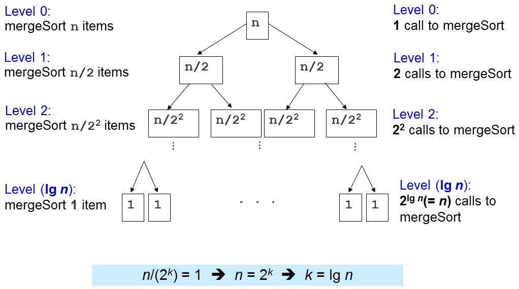
(Image source: https://visualgo.net/img/merge.png)

Time complexity and Space complexity

• Time complexity: Θ(nLog(n)) is the time complexity of the merge sort in all 3 cases(average, worst, and best) 

• Space complexity: O(n)  It uses additional memory for left and right sub arrays. Hence, total O(n) extra memory is needed for the array of n size.

Drawbacks of merge sort:

• It is a slow algorithm than other sorting algorithms to perform smaller tasks.
• It goes through the whole process even if the array is sorted.
• Merge sort requires extra space O(n)  to store temporary arrays.

Quick Sort

• It is also a famous sorting algorithm.
• It uses a divide and conquer paradigm for sorting.
• It is not a stable sort.
• It is in-place sort.
• It divides the given array into two sections using a partitioning element called a pivot.
• All the elements to the left side of the pivot are smaller than the pivot.
• All the elements to the right side of the pivot are greater than the pivot.

Time complexity and Space complexity

• Best Case Time complexity: O(nLog(n))  The best case occurs when the pivot element is always in the middle of the array.

• Worst Case Time complexity: O(n^2)  when the array is already sorted in increasing or decreasing order, then it divides the array into sections of 1 and (n-1) elements in each call. Therefore, here total comparisons required are f(n) = n * (n-1) = O(n²).

• Space complexity: O(nLog(n)): In the average case space used will be of the order O(nLog(n)) and for the worst case, the space complexity becomes O(n).

Counting Sort

• Counting sort is a stable technique, 
• It is not a comparison based algorithm like other sorting algorithms(bubble, selection, insertion, merge, etc...).

Time complexity and Space complexity

• Time complexity:O(n+k) is the time complexity of counting sort where n is the number of elements in the input array and k is the range of input. 
• Space complexity: O(n+k) space to hold the indices, counts, and output array.

Drawbacks of merge sort:

• It is not suitable for sorting large data sets.

• It will not work if we have 5 elements to sort in the range of 0 to 10,000.

• It is not suitable for sorting string values.

Radix Sort

• radix sort can be used for sorting numbers having a large range, unlike counting sort.
• Fast when the keys are short i.e. when the range of the array elements is less.
• it takes more space than Quick Sort.

Time complexity and Space complexity

• Time complexity: O(l*(n+k)) where n$n$ is the number of items to sort, $\ell$l is the number of digits in each item, and $k$ is the number of values each digit can have. 
• We're calling counting sort one time for each of the l digits in the input numbers, and the counting sort has a time complexity of O(n + k). So, the time complexity of radix sort will be O(l*(n+k)).
• Space complexity: O(n+k) space to hold the indices, counts, and output array.

Heap Sort

• Heap is an almost complete binary tree, the last level is strictly filled from left to right.
• Binary Heap is of two types- 1. Max Heap (every node contains greater or equal value element than all its descendants.) 2. Min Heap (every node contains a smaller value element than all its descendants.)
• Heap Sort is not a Stable Algorithm but it is an in-place algorithm.
• It is an efficient algorithm, increases logarithmically.
• Heap sort algorithm has limited uses because Quicksort and mergesort are better in practice.

Time complexity and Space complexity

• Time complexity:O(nLog(n)) Time complexity of createAndBuildHeap() is O(n) and the overall time complexity of Heap Sort is O(nLog(n)).
• Space complexity: O(1)

   "HEAP SORT uses MAX_HEAPIFY function which calls itself but it can be made using a simple while loop and thus making it an iterative function which inturn takes no space and hence Space Complexity of HEAP SORT can be reduced to O(1)."

   

Bucket Sort

for floating-point numbers:

• Bucket sort is mainly used when input is uniformly distributed over a range.
• When the large array of floating-point numbers are given then bucket sort is the efficient way to sort an array within the O(n) time complexity, other algorithms such as Merge Sort, Quick Sort, etc... can't do better than O(nLog(n)). 

Algorithm :

bucketSort(arr[], n)
1) Create n empty buckets (Or lists).
2) Do following for every array element arr[i].
.......a) Insert arr[i] into bucket[n*array[i]]
3) Sort individual buckets using insertion sort.
4) Concatenate all sorted buck

Time complexity 

• Time complexity: O(n)  If we assume that insertion in a bucket takes O(1) time then steps 1 and 2 of the above algorithm clearly take O(n) time. 

for integer numbers

Time complexity and Space complexity

• Time complexity: O(n+k)  If we assume that insertion in a bucket takes O(1) time then steps 1 and 2 of the above algorithm clearly take O(n) time. 
• Worst Case Time complexity: O(n^2)
• Space complexity: O(nk) for the worst case